Maximum likelihood
In Bayesian modelling, the likelihood,  , is the name given to the measure of the goodness of fit between the model, with some given variables, and the data. When the likelihood is maximised,
  , the most probable statistical model has been found for the given data.
In this tutorial we will see how uravu can be used to maximize the likelihood of a model for some dataset.
In uravu, when the sample is normally distributed the likelihood is calculated as follows,
![\ln L = -0.5 \sum_{i=1}^n \bigg[ \frac{(y_i - m_i) ^2}{\delta y_i^2} + \ln(2 \pi \delta y_i^2) \bigg],](_images/math/2286e0c11a0245187a7189e0fde4285eb97b7ef3.png)
where,  is the data ordinate,
  is the model ordinate, and
  is uncertainty in .
 uravu is able to maximize this function using the scipy.optimize.minimize() function (we minimize the negative of the likelihood).
Before we maximise the likelihood, is it necessary to create some synthetic data to analyse.
[1]:
import numpy as np
import matplotlib.pyplot as plt
from uravu import plotting
from uravu.relationship import Relationship
[2]:
np.random.seed(1)
[3]:
x = np.linspace(0, 10, 20)
y = np.exp(0.5 * x) * 4
y += y * np.random.randn(20) * 0.1
dy = y * 0.2
[4]:
plt.errorbar(x, y, dy, marker='o', ls='')
plt.yscale('log')
plt.show()
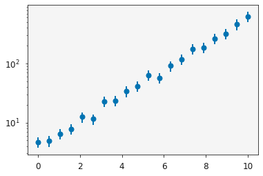
The data plotted above (note the logarthimic -axis) may be modelled with the following relationship,
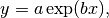
where  and
and  are the variables of interest in the modelling process. We want to find the values for these variables, which maximises the likelihood.
First, we must write a function to describe the model (more about the function specification can be found in teh Input functions tutorial).
[5]:
def my_model(x, a, b):
    """
    A function to describe the model under investgation.

    Args:
        x (array_like): Abscissa data.
        a (float): The pre-exponential factor.
        b (float): The x-multiplicative factor.

    Returns
        y (array_like): Ordinate data.
    """
    return a * np.exp(b * x)
With our model defined, we can construct a Relationship object.
[6]:
modeller = Relationship(my_model, x, y, ordinate_error=dy)
The Relationship object gives us access to a few powerful Bayesian modelling methods. However, this tutorial is focused on maximising the likelihood, this is achieved with the max_likelihood() class method, where the keyword 'mini' indicates the standard scipy.optimize.minimize() function should be used.
[7]:
modeller.max_likelihood('mini')
[8]:
print(modeller.variable_modes)
[4.55082086 0.46090669]
We can see that the variables are close to the values used in the data synthesis. Note, that here variable_modes are in fact the variable values that maximise the likelihood.
Let’s inspect the model visually. This can be achieved easily with the plotting module in uravu.
[9]:
ax = plotting.plot_relationship(modeller)
plt.yscale('log')
plt.show()
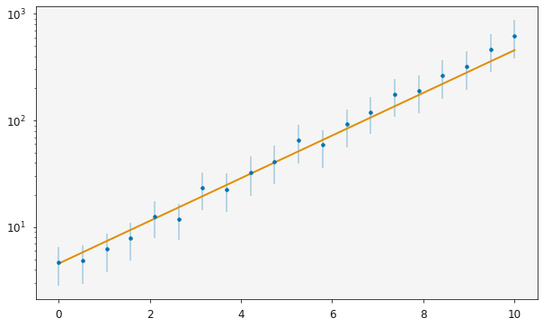
Above, we can see that the orange line of maximum likelihood agrees well with the data.