Getting started

uravu enables the use of powerful Bayesian modelling in Python, building on the capabilities of emcee and dynesty, for the understanding of some data. To show how this can be used, we will create some synthetic data using numpy.

import numpy as np
import matplotlib.pyplot as plt
from uravu.relationship import Relationship
from uravu import plotting

np.random.seed(1)

x = np.linspace(0, 9, 10)
y = np.linspace(0, 18, 10) + 2
y += y * np.random.randn((10)) * 0.025
y_err = np.ones((10))

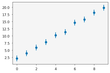
Plotting this data, shows it appears to be a straight line relationship, with some gradient and intercept.

plt.errorbar(x, y, y_err, marker='o', ls='')
plt.show()

Let’s use uravu to model a straight line function for the data, for more information about the requirements of the input function check out the Input functions tutorial.

def straight_line(x, m, c):
    """
    A straight line.

    Args:
        x (array_like): Abscissa data.
        m (float): Gradient.
        c (float): Intercept.

    Returns:
        (array_like): Ordinate data.
    """
    return m * x + c

The function, x data, y data, and y error can then be brought together in the Relationship class.

modeller = Relationship(straight_line, x, y, ordinate_error=y_err)

The Relationship class enables substantial functionality and is at the core of uravu, you can learn about this functionality in the tutorials. Quickly, we will show the maximisation of the likelihood (there is more about this in the first tutorial).

modeller.max_likelihood('mini')

The string 'mini' indicates that the standard scipy.optimize.minimize() function should be used.

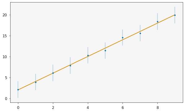
The built in plotting library can be used to make publication quality plot of the Relationship.

fig, ax = plt.subplots(figsize=(10, 6))
ax = plotting.plot_relationship(modeller, axes=ax)
plt.show()

We hope you enjoy using uravu, feel free to contribute on Github, and tell your friends and colleagues!