Nested sampling¶

In the MCMC tutorial, Bayes theorem was shown,

$p = \frac{P L}{Z},$

where where, $p$ is the posterior probability, $P$ is the prior probability, $L$ is the likelihood, and $Z$ is the evidence. Normally, in the evaluation of the posterior probability, the evidence is removed as a constant of proportionality. This is due to the fact that it is a single value for a given model and dataset pair.

However, sometimes it is desirable to find the evidence for a model to a given dataset. In particular, when we want to compare the evidence for a series of models, to determine which best describes the dataset. In order to achieve this, uravu is able to perform nested sampling to estimate the Bayesian evidence for a model given a particular dataset.

This tutorial will show how this is achieved, and show the utility of Bayesian model selection.

However, as always we must first create some synthetic data.

[1]:

import numpy as np
import matplotlib.pyplot as plt
from scipy.stats import lognorm
from uravu.distribution import Distribution
from uravu.relationship import Relationship
from uravu import plotting, utils

[2]:

np.random.seed(2)

This synthetic data is log-normally distributed in the ordinate. Below, we use a scipy.stats.rv_continuous object to define our ordinate data.

[6]:

x = np.linspace(10, 50, 20)
y = .3 * x ** 2 - 1.4 * x + .2
Y = []
for i in y:
    Y.append(lognorm(s=2, loc=i, scale=1))

From looking at the code used to synthesize this data, it is clear that the functional form of the model is a second order polynomial. However, if this was data collected from some measurement and the physical theory suggests it should be analysed with a polynormial of unknown degree then Bayesian model selection would be the ideal tool to find the best model.

Let’s quickly write a few models to perform the n degree polynomial analysis with.

[7]:

def one_degree(x, a, b):
    return b * x + a

def two_degree(x, a, b, c):
    return c * x ** 2 + b * x + a

def three_degree(x, a, b, c, d):
    return d * x ** 3 + c * x ** 2 + b * x + a

def four_degree(x, a, b, c, d, e):
    return e * x ** 4 + d * x ** 3 + c * x ** 2 + b * x + a

With these functions defined, we can now build the Relationship objects for each of the functions. Using the 'diff_evo' string to perform the global optimisation by differential evolution.

[8]:

one_modeller = Relationship(one_degree, x, Y,
                            bounds=((-300, 0), (-2, 20)))
one_modeller.max_likelihood('diff_evo')

[9]:

two_modeller = Relationship(two_degree, x, Y,
                            bounds=((-2, 2), (-2, 2), (-1, 1)))
two_modeller.max_likelihood('diff_evo')

[10]:

three_modeller = Relationship(three_degree, x, Y,
                              bounds=((-2, 2), (-2, 2), (-1, 1), (-0.2, 0.2)))
three_modeller.max_likelihood('diff_evo')

[11]:

four_modeller = Relationship(four_degree, x, Y,
                             bounds=((-2, 2), (-2, 2), (-1, 1), (-0.2, 0.2), (-0.02, 0.02)))
four_modeller.max_likelihood('diff_evo')

Having built these, lets see what the maximum likelihood variables are for each.

[12]:

print(one_modeller.variable_modes)

[-233.02181382   16.91419436]

[13]:

print(two_modeller.variable_modes)

[ 0.50360562 -1.22086729  0.29722928]

[14]:

print(three_modeller.variable_modes)

[-3.41783502e-01 -1.19673254e+00  2.97185414e-01 -8.76900188e-07]

[15]:

print(four_modeller.variable_modes)

[ 1.20603075e+00  4.35409450e-01  1.48054997e-01  4.14102794e-03
 -3.65616682e-05]

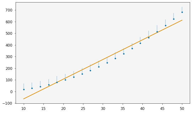
It is possible to quickly visualise the relationship with the plotting function, which shows the log-normal distribution of the ordinate data.

[16]:

plotting.plot_relationship(one_modeller)
plt.show()

Above, in the variable_modes, we can see that the highest order terms are quite small for the larger degree of polynomial. Let’s see what effect this has on the evidence.

Note that uravu and dynesty calculates the natural log of the evidence, $\ln{Z}$ and while this tutorial show how nested sampling may be used, uravu and dynesty also enable the use of dynamic nested sampling (by setting the keyword argument dynamic to True).

[17]:

one_modeller.nested_sampling()

3281it [00:20, 158.05it/s, +500 | bound: 5 | nc: 1 | ncall: 20604 | eff(%): 18.351 | loglstar:   -inf < -110.062 <    inf | logz: -115.772 +/-  0.137 | dlogz:  0.001 >  0.509]

[18]:

two_modeller.nested_sampling()

3495it [00:25, 138.14it/s, +500 | bound: 6 | nc: 1 | ncall: 21404 | eff(%): 18.665 | loglstar:   -inf < -82.411 <    inf | logz: -88.545 +/-  0.142 | dlogz:  0.001 >  0.509]

[19]:

three_modeller.nested_sampling()

5843it [00:37, 154.48it/s, +500 | bound: 15 | nc: 1 | ncall: 28341 | eff(%): 22.381 | loglstar:   -inf < -84.331 <    inf | logz: -95.193 +/-  0.200 | dlogz:  0.001 >  0.509]

[20]:

four_modeller.nested_sampling()

8725it [01:01, 140.73it/s, +500 | bound: 29 | nc: 1 | ncall: 39087 | eff(%): 23.601 | loglstar:   -inf < -83.449 <    inf | logz: -100.113 +/-  0.254 | dlogz:  0.001 >  0.509]

Having estimated $\ln{Z}$ for each Relationship, lets plot them as a function of the number of variables in the model.

[21]:

variables = [len(one_modeller.variables), len(two_modeller.variables),
             len(three_modeller.variables), len(four_modeller.variables)]
ln_evidence = [one_modeller.ln_evidence.n, two_modeller.ln_evidence.n,
               three_modeller.ln_evidence.n, four_modeller.ln_evidence.n]
ln_evidence_err = [one_modeller.ln_evidence.s, two_modeller.ln_evidence.s,
                   three_modeller.ln_evidence.s, four_modeller.ln_evidence.s]

[22]:

plt.errorbar(variables, ln_evidence, ln_evidence_err, marker='o', ls='')
plt.xlabel('Number of variables')
plt.ylabel(r'$\ln{Z}$')
plt.show()

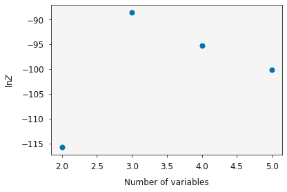
We can see that the evidence reaches a maxiumum at 3 variables (the two_degree model), this indicates that this is the most probable model for analysis of this dataset.

Finally, we can use some built in functionality of uravu to compare different evidence values, in a value known as the Bayes factor. Let’s compare the one_degree and two_degree models.

[23]:

print(utils.bayes_factor(two_modeller.ln_evidence, one_modeller.ln_evidence))

54.5+/-0.4

The Bayes factor between the two and one degree models, $2\ln{B_{21}}$ , has a value of $\sim81$ . The Table in Kass and Raftery suggests that this shows “Strong” evidence for the model with more variables (the two_degree model).

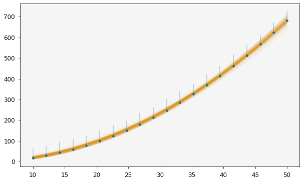
This means that it is sensible to go ahead and use the two_degree model in the further analysis of our data. Below the plot of the second order polynomial is shown over the data.

[24]:

plotting.plot_relationship(two_modeller)
plt.show()

[ ]: